Multi Phase Orientation Mapping

You can also calculate the orientation of the grains for multiple phases using the pyxem.signals.PolarSignal2D.get_orientation() method. This requires that you simulate the entire S2 space for the phase and then compare to the simulated diffraction.

For more information on the orientation mapping process see [CCAAnes+22]

import pyxem as pxm
from pyxem.data import fe_multi_phase_grains, fe_bcc_phase, fe_fcc_phase
from diffsims.generators.simulation_generator import SimulationGenerator
from orix.quaternion import Rotation
from orix.sampling import get_sample_reduced_fundamental
import hyperspy.api as hs

multi_phase = fe_multi_phase_grains()

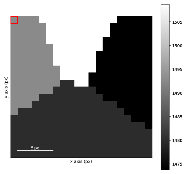
First we center the diffraction patterns and get a polar signal Increasing the number of npt_azim with give better polar sampling but will take longer to compute the orientation map The mean=True argument will return the mean pixel value in each bin rather than the sum this makes the high k values more visible

multi_phase.calibration.center = None
polar_multi = multi_phase.get_azimuthal_integral2d(
    npt=100, npt_azim=360, inplace=False, mean=True
)
polar_multi.plot()

• 
• 

  0%|          | 0/17 [00:00<?, ?it/s]
 35%|███▌      | 6/17 [00:00<00:00, 32.50it/s]
 59%|█████▉    | 10/17 [00:00<00:00, 28.42it/s]
 76%|███████▋  | 13/17 [00:00<00:00, 27.85it/s]
 94%|█████████▍| 16/17 [00:00<00:00, 23.44it/s]
100%|██████████| 17/17 [00:00<00:00, 26.51it/s]

Now we can get make a simulation. In this case we want to set a minimum_intensity which removes the low intensity reflections. We also sample the S2 space using the orix.sampling.get_sample_reduced_fundamental() We have two phases here so we can make a simulation object with both of the phases.

bcc = fe_bcc_phase()
fcc = fe_fcc_phase()
bcc.name = "BCC Phase"
fcc.name = "FCC Phase"
fcc.color = "red"
bcc.color = "blue"

generator = SimulationGenerator(200, minimum_intensity=0.05)
rotations_bcc = get_sample_reduced_fundamental(
    resolution=1, point_group=bcc.point_group
)
rotations_fcc = get_sample_reduced_fundamental(
    resolution=1, point_group=fcc.point_group
)

sim = generator.calculate_diffraction2d(
    [bcc, fcc],
    rotation=[rotations_bcc, rotations_fcc],
    max_excitation_error=0.1,
    reciprocal_radius=2,
    with_direct_beam=False,
)

Orientation Mapping

Now we can calculate the orientation map using the polar signal and the simulated diffraction pattern Sometimes a gamma correction helps to re-normalize the intensity of the simulated diffraction pattern and increase the intensity of the high k diffraction spots. Unfortunately this is quite dependent on the detector response/ sample thickness etc. As a result there is no good rule of thumb. As such it is important to play with this value/ use the background correction to get the best results. Additionally, here we have set the n_best to -1 which means that we will return all the orientations in the simulation. This is not always the best option as it can lead to memory spikes. It does allow us to plot a very nice heatmap of the orientation. Which is useful for understanding the orientation mapping process and mis-orientations.

polar_multi = polar_multi**0.5  # gamma correction
orientation_map = polar_multi.get_orientation(sim, n_best=-1, frac_keep=1)

  0%|          | 0/17 [00:00<?, ?it/s]
  6%|▌         | 1/17 [00:00<00:01,  8.56it/s]
 12%|█▏        | 2/17 [00:00<00:02,  5.25it/s]
 18%|█▊        | 3/17 [00:00<00:02,  6.45it/s]
 24%|██▎       | 4/17 [00:00<00:02,  5.32it/s]
 29%|██▉       | 5/17 [00:00<00:01,  6.22it/s]
 35%|███▌      | 6/17 [00:01<00:04,  2.38it/s]
 41%|████      | 7/17 [00:01<00:03,  3.06it/s]
 47%|████▋     | 8/17 [00:02<00:03,  2.99it/s]
 53%|█████▎    | 9/17 [00:02<00:03,  2.48it/s]
 59%|█████▉    | 10/17 [00:03<00:03,  2.31it/s]
 65%|██████▍   | 11/17 [00:03<00:02,  2.13it/s]
 71%|███████   | 12/17 [00:04<00:02,  2.31it/s]
 76%|███████▋  | 13/17 [00:04<00:01,  2.89it/s]
 82%|████████▏ | 14/17 [00:05<00:01,  1.94it/s]
 88%|████████▊ | 15/17 [00:05<00:00,  2.48it/s]
 94%|█████████▍| 16/17 [00:05<00:00,  2.37it/s]
100%|██████████| 17/17 [00:05<00:00,  2.90it/s]

  0%|          | 0/17 [00:00<?, ?it/s]
100%|██████████| 17/17 [00:00<00:00, 1636.22it/s]

Plotting The Orientation Mapping

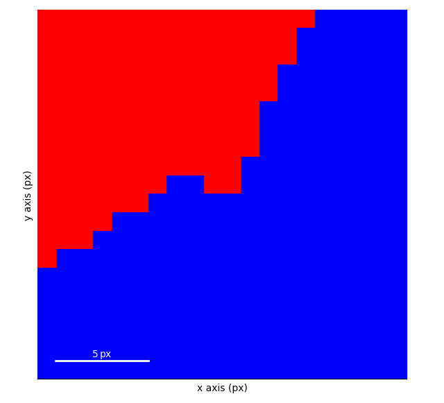
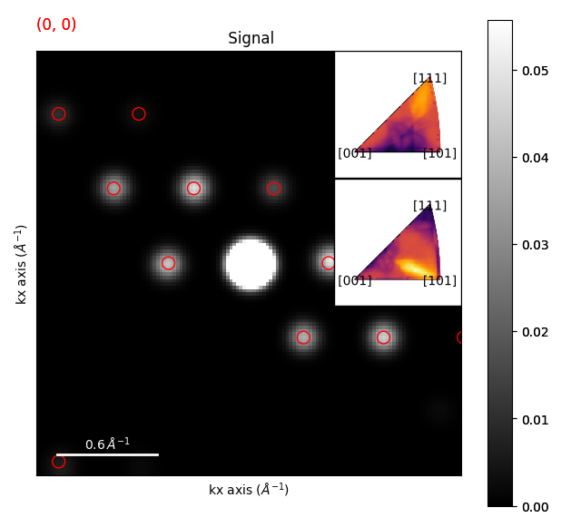
We can then plot the orientation map using the pyxem.signals.OrientationMap.plot_over_signal() method. Here we have set add_ipf_correlation_heatmap=True which will add a heatmap of the IPF correlation.

orientation_map.plot_over_signal(
    multi_phase, vmax="99th", add_ipf_correlation_heatmap=True
)

• 
• 

  0%|          | 0/33 [00:00<?, ?it/s]
100%|██████████| 33/33 [00:00<00:00, 3369.74it/s]

  0%|          | 0/33 [00:00<?, ?it/s]
100%|██████████| 33/33 [00:00<00:00, 3571.00it/s]

  0%|          | 0/49 [00:00<?, ?it/s]
100%|██████████| 49/49 [00:00<00:00, 846.01it/s]

  0%|          | 0/49 [00:00<?, ?it/s]
100%|██████████| 49/49 [00:00<00:00, 738.41it/s]

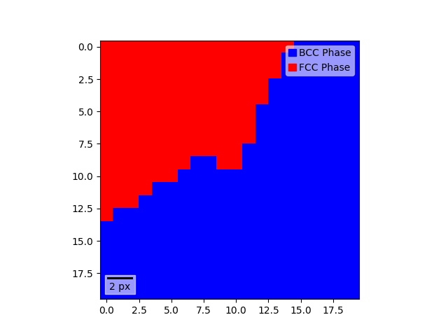
Getting the Crystal Map

Now we can calculate the orientation map using the polar signal and the simulated diffraction pattern Sometimes a gamma correction helps to re-normalize the intensity of the simulated diffraction pattern and increase the intensity of the high k diffraction spots. Unfortunately this is quite dependent on the detector response/ sample thickness etc. As a result there is no good rule of thumb. As such it is important to play with this value/ use the background correction to get the best results.

cmap = orientation_map.to_crystal_map()
cmap.plot()

  0%|          | 0/33 [00:00<?, ?it/s]
 45%|████▌     | 15/33 [00:00<00:00, 140.58it/s]
 91%|█████████ | 30/33 [00:00<00:00, 112.95it/s]
100%|██████████| 33/33 [00:00<00:00, 108.37it/s]

  0%|          | 0/33 [00:00<?, ?it/s]
100%|██████████| 33/33 [00:00<00:00, 3004.32it/s]

sphinx_gallery_thumbnail_number = 4