Clustering Vectors

This can be used to segment a 4-D STEM dataset into different clusters based on the diffraction pattern at each real space position.

import pyxem as pxm
from scipy.ndimage import gaussian_filter
import matplotlib.pyplot as plt
from sklearn.cluster import DBSCAN

# Getting the vectors for some dataset
# s = pxm.data.mgo_nanocrystals(allow_download=True)
s = pxm.data.simulated_overlap()
s.filter(gaussian_filter, sigma=(0.5, 0.5, 0, 0), inplace=True)  # only in real space
s.template_match_disk(disk_r=5, subtract_min=False, inplace=True)
vectors = s.get_diffraction_vectors(threshold_abs=0.5, min_distance=3)

# Now we can convert the vectors into a 2D array of rows/columns
flat_vectors = (
    vectors.flatten_diffraction_vectors()
)  # flatten the vectors into a 2D array
scan = DBSCAN(eps=1.0, min_samples=2)

/home/docs/checkouts/readthedocs.org/user_builds/pyxem/envs/1139/lib/python3.11/site-packages/diffsims/generators/sphere_mesh_generators.py:523: RuntimeWarning: invalid value encountered in divide
  phi2 = sign * np.nan_to_num(np.arccos(x_comp / norm_proj))

  0%|          | 0/9 [00:00<?, ?it/s]
 11%|█         | 1/9 [00:01<00:12,  1.53s/it]
 33%|███▎      | 3/9 [00:03<00:05,  1.03it/s]
 56%|█████▌    | 5/9 [00:04<00:03,  1.16it/s]
 78%|███████▊  | 7/9 [00:06<00:01,  1.21it/s]
100%|██████████| 9/9 [00:06<00:00,  1.46it/s]

  0%|          | 0/17 [00:00<?, ?it/s]
  6%|▌         | 1/17 [00:01<00:16,  1.02s/it]
 29%|██▉       | 5/17 [00:02<00:04,  2.59it/s]
 41%|████      | 7/17 [00:02<00:02,  3.64it/s]
 53%|█████▎    | 9/17 [00:03<00:02,  2.93it/s]
 76%|███████▋  | 13/17 [00:04<00:01,  3.49it/s]
100%|██████████| 17/17 [00:04<00:00,  4.08it/s]

  0%|          | 0/33 [00:00<?, ?it/s]
100%|██████████| 33/33 [00:00<00:00, 552.67it/s]

Clustering the Vectors

It is very important that we first normalize the real and reciprocal space distances The column scale factors map the real space and reciprocal space distances to the same scale Here this means that the clustering algorithm operates on 4 nm in real space and .1 nm^-1 in reciprocal space based on the units for the vectors.

clustered = flat_vectors.cluster(
    scan,
    column_scale_factors=[2, 2, 0.05, 0.05],
    columns=[0, 1, 2, 3],
    min_vectors=40,
)
m, p = clustered.to_markers(s, alpha=0.8, get_polygons=True)
s.plot()
s.add_marker(m)
s.add_marker(p, plot_on_signal=False)

• 
• 

  0%|          | 0/2 [00:00<?, ?it/s]
 50%|█████     | 1/2 [00:00<00:00,  2.07it/s]
100%|██████████| 2/2 [00:00<00:00,  4.13it/s]

vect = clustered.map_vectors(
    pxm.utils.vectors.column_mean,
    columns=[0, 1],
    label_index=-1,
    dtype=float,
    shape=(2,),
)
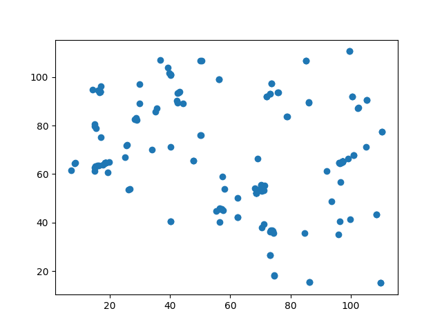
plt.figure()
plt.scatter(vect[:, 1], vect[:, 0])

/home/docs/checkouts/readthedocs.org/user_builds/pyxem/envs/1139/lib/python3.11/site-packages/numpy/_core/fromnumeric.py:3860: RuntimeWarning: Mean of empty slice.
  return _methods._mean(a, axis=axis, dtype=dtype,
/home/docs/checkouts/readthedocs.org/user_builds/pyxem/envs/1139/lib/python3.11/site-packages/numpy/_core/_methods.py:137: RuntimeWarning: invalid value encountered in divide
  ret = um.true_divide(

<matplotlib.collections.PathCollection object at 0x7588bfd4fa10>

clusterer = DBSCAN(min_samples=2, eps=4)

clustered2 = clustered.cluster_labeled_vectors(method=clusterer)
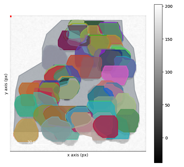
m, p = clustered2.to_markers(s, alpha=0.8, get_polygons=True)

36 : Clusters Found!

Visualizing the Clustering

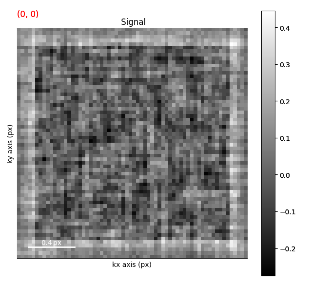
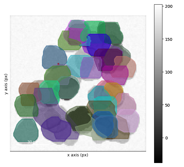
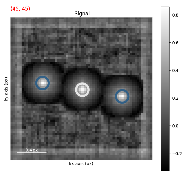
This clustering is works pretty good after the second step. We can interact with the results as well in order to see regions where the clustering doesn’t work quite as well!

m, p = clustered2.to_markers(
    s, alpha=0.8, get_polygons=True, facecolor="none", sizes=(30,), lw=5
)
s.axes_manager.indices = (45, 45)
s.plot()
s.add_marker(m)
s.add_marker(p, plot_on_signal=False)
# sphinx_gallery_thumbnail_number = 5

• 
•