Centering the Zero Beam

Making a Dummy Dataset with a Zero Beam that systematically deviates from the center

import hyperspy.api as hs
import pyxem as pxm

s = pxm.data.tilt_boundary_data(correct_pivot_point=False)

  0%|          | 0/49 [00:00<?, ?it/s]
100%|██████████| 49/49 [00:00<00:00, 766.69it/s]

Getting the Position of the Zero beam

The zero beam position can be obtained using the get_direct_beam_position() method.

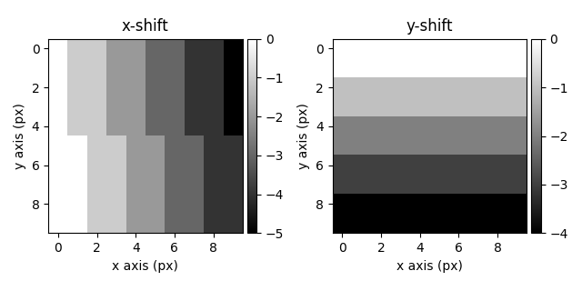
s_shifts = s.get_direct_beam_position(method="blur", sigma=5, half_square_width=20)
s_shifts.plot()

# Getting a Linear Plane
# ---------------------
# In many instances the zero beam position will vary systematically with the scan position.
# This can be corrected by fitting a linear plane to the zero beam position using the
# :meth:`get_linear_plane` method.
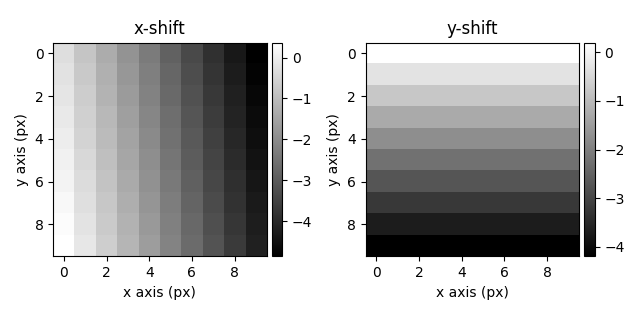
s_linear_plane = s_shifts.get_linear_plane()
s_linear_plane.plot()

• 
• 

  0%|          | 0/33 [00:00<?, ?it/s]
100%|██████████| 33/33 [00:00<00:00, 1434.69it/s]

[<Axes: title={'center': 'x-shift'}, xlabel='x axis (px)', ylabel='y axis (px)'>, <Axes: title={'center': 'y-shift'}, xlabel='x axis (px)', ylabel='y axis (px)'>]

Centering the Zero Beam

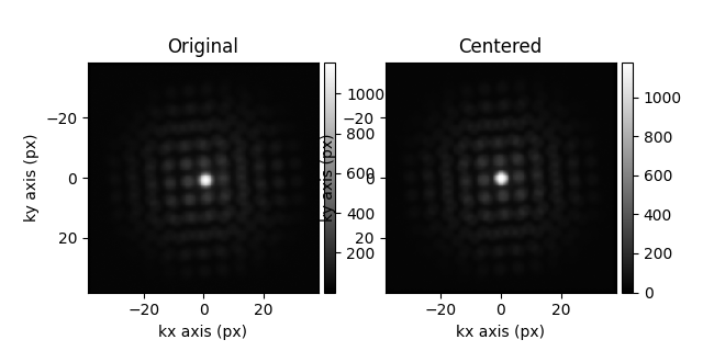
The zero beam can be centered using the center_direct_beam() method. Then we sum all the diffraction patterns for the both the centered beam, and the non-centered one, to compare them.

s_centered = s.center_direct_beam(shifts=s_linear_plane, inplace=False)
s_pacbed_centered = s_centered.sum()
s_pacbed = s.sum()

hs.plot.plot_images([s_pacbed, s_pacbed_centered], label=["Original", "Centered"])

  0%|          | 0/49 [00:00<?, ?it/s]
100%|██████████| 49/49 [00:00<00:00, 749.24it/s]

[<Axes: title={'center': 'Original'}, xlabel='kx axis (px)', ylabel='ky axis (px)'>, <Axes: title={'center': 'Centered'}, xlabel='kx axis (px)', ylabel='ky axis (px)'>]

Centering the Zero Beam with constant deflection magnitude

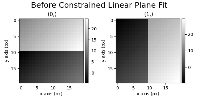
In the presence of electromagnetic fields in the entire sample area, the plane fitting can fail. In this case, two separate effects can be observed:

1. The zero beam position varies systematically with the scan position due to the effects of descan

2. The zero beam will be deflected from electromagnetic fields in the sample

Assuming that the effects of 1 are systematic and that the electromagnetic fields have constant strengths, we can try to fit a plane to correct for effects of 1 by minimizing the magnitude variance. You may need use a mask and/or have several electromagnetic domains for good performance.

s_probes = pxm.data.simulated_constant_shift_magnitude()

s_shifts = s_probes.get_direct_beam_position(method="center_of_mass")

  0%|          | 0/49 [00:00<?, ?it/s]
100%|██████████| 49/49 [00:00<00:00, 701.77it/s]

Getting the Linear Plane

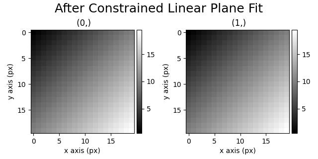
We call get_linear_plane with constrain_magnitude_variance=True. Then we can center the direct beam as normal.

s_shifts.plot(suptitle="Before Constrained Linear Plane Fit")
s_linear_plane = s_shifts.get_linear_plane(constrain_magnitude_variance=True)
s_linear_plane.plot(suptitle="After Constrained Linear Plane Fit")

s_probes.center_direct_beam(shifts=s_linear_plane)

• 
• 

  0%|          | 0/49 [00:00<?, ?it/s]
100%|██████████| 49/49 [00:00<00:00, 713.65it/s]

Getting the Electromagnetic Domains

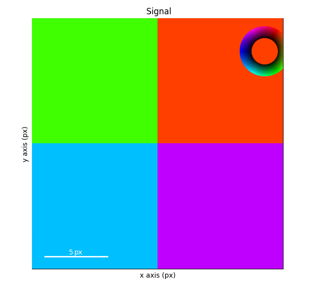
The found electromagnetic domains can be visualized by subtracting the linear plane from the original shifts. This is done by subtracting the linear plane determined from the constrained magnitude variance from the original shifts.

s_shifts -= s_linear_plane
s_shifts.get_magnitude_phase_signal().plot()

# For more realistic data, the linear plane optimization algorithm can give poor results. In this case,
# you can change the initial values for the optimization algorithm by using the `initial_values` parameter
# in `get_linear_plane`. See the docstring for more information. Try varying this and see if the plane
# changes significantly.