Calibrating Scales

This example demonstrates how to calibrate the scales in both reciprocal and real-space. Ideally this should be done using a calibration standard with a known lattice spacing.

There are many ways to calibrate the microscope so raise an issue if you have a specific method you would like to see implemented or if you have any questions.

from diffsims.generators.simulation_generator import SimulationGenerator
import pyxem as pxm
import hyperspy.api as hs
import numpy as np
from diffsims.utils.sim_utils import get_electron_wavelength
from scipy.optimize import curve_fit
import matplotlib.pyplot as plt


# Load the data and the cif file
au_dpeg = pxm.data.au_grating_20cm(
    allow_download=True, signal_type="electron_diffraction"
)
gold_phase = pxm.data.au_phase(allow_download=True)  # Orix.CrystalMap.Phase object

  0%|                                               | 0.00/263k [00:00<?, ?B/s]
  5%|██▏                                    | 14.3k/263k [00:00<00:01, 136kB/s]
 15%|█████▉                                 | 39.9k/263k [00:00<00:01, 199kB/s]
 41%|████████████████▍                       | 108k/263k [00:00<00:00, 405kB/s]
 68%|███████████████████████████▏            | 178k/263k [00:00<00:00, 509kB/s]
  0%|                                               | 0.00/263k [00:00<?, ?B/s]
100%|███████████████████████████████████████| 263k/263k [00:00<00:00, 2.13GB/s]

  0%|                                              | 0.00/4.58k [00:00<?, ?B/s]
  0%|                                              | 0.00/4.58k [00:00<?, ?B/s]
100%|█████████████████████████████████████| 4.58k/4.58k [00:00<00:00, 43.8MB/s]

Create a Simulation Generator

Use the SimulationGenerator to create a simulated diffraction pattern from the gold phase. Note that the acceleration voltage is irrelevant

sim_gen = SimulationGenerator()
sim1d = sim_gen.calculate_diffraction1d(gold_phase, reciprocal_radius=1.2)

Azimuthal Integration and Calibration

The polar unwrapping for the 2D image will give a 1D diffraction pattern that can be used for calibration. The calibration is done by comparing the positions of the peaks in the simulated and experimental diffraction patterns. Fitting with a hyperspy.model.Model1D can be used to find the scale or the camera length.

au_dpeg.calibration.center = None  # Set the center
az1d = au_dpeg.get_azimuthal_integral1d(npt=200, radial_range=(20, 128))  # in pixels
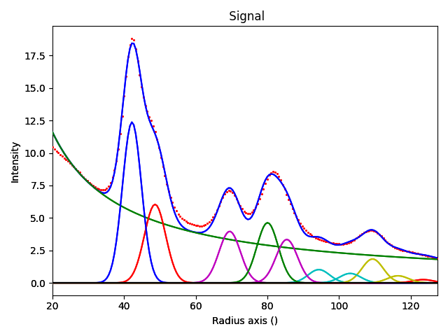
diffraction_model = az1d.model_simulation1d(sim1d, fit=True, center_lim=0.03)

theta_scale = az1d.model2theta_scale(
    simulation=sim1d, model=diffraction_model, beam_energy=200
)

camera_length = az1d.model2camera_length(
    simulation=sim1d,
    model=diffraction_model,
    beam_energy=200,
    physical_pixel_size=5.5e-5,
)

print("Theta Scale: ", theta_scale, " Rad")
print(
    "Camera Length: ", camera_length * 100, " cm"
)  # Camera length of 21.287cm (vs 20cm from the microscope)
diffraction_model.plot(plot_components=True)

  0%|          | 0/2 [00:00<?, ?it/s]
100%|██████████| 2/2 [00:00<00:00, 1154.50it/s]
Theta Scale:  0.0002542800394167303  Rad
Camera Length:  21.6296957247437  cm

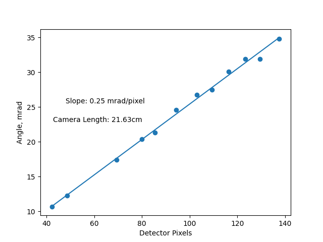
Aside: Showing how the Camera Length and scale is caluclated:

centers = np.sort(
    [
        c.centre.value
        for c in diffraction_model
        if isinstance(c, hs.model.components1D.Gaussian)
    ]
)
wavelength = get_electron_wavelength(200)
angles = np.arctan2(
    np.sort(sim1d.reciprocal_spacing), 1 / wavelength
)  # both in inverse angstroms.


def f(x, m):
    return x * m


m, pcov = curve_fit(f, centers, angles)
scale = m[0]

fig, axs = plt.subplots(1)
axs.scatter(centers, angles * 1000)
axs.plot(np.sort(centers), np.sort(centers) * scale * 1000)
axs.set_ylabel("Angle, mrad")
axs.set_xlabel("Detector Pixels")
axs.annotate(f"Slope: {scale*1000:.2} mrad/pixel", (0.1, 0.6), xycoords="axes fraction")
axs.annotate(
    f"Camera Length: {5.5E-5/ np.tan(scale)*100:.4}cm",
    (0.05, 0.5),
    xycoords="axes fraction",
)

Text(0.05, 0.5, 'Camera Length: 21.63cm')

Applying a Camera Length

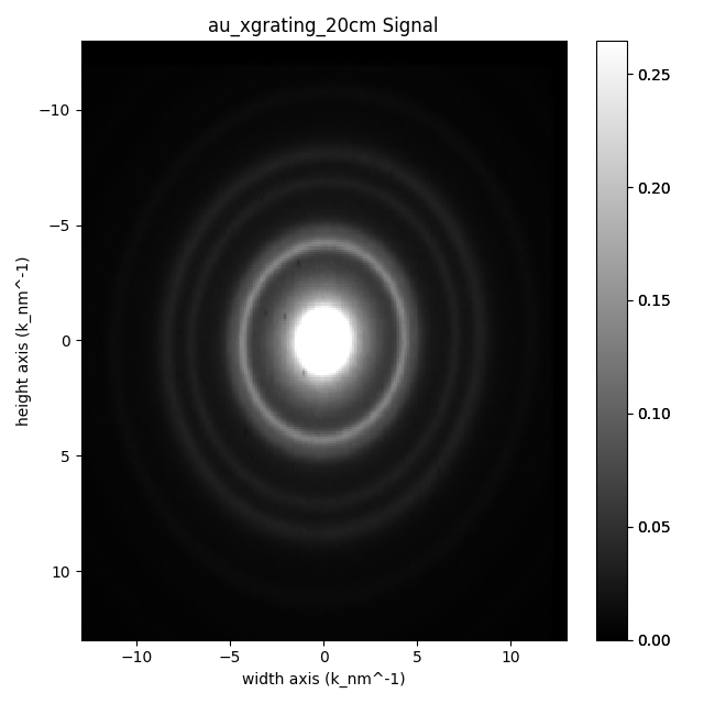
The (calibrated) camera length can be applied to the data to calibrate the scale more accurately than a simple single point calibration. Let’s apply the camera length to the data and plot the result.

au_dpeg.calibration.detector(
    pixel_size=5.5e-5, detector_distance=camera_length, beam_energy=200
)
print(au_dpeg.axes_manager)  # non uniform axes
au_dpeg.plot(vmax="99th")  # non uniform axes

<Axes manager, axes: (|256, 256)>
            Name |   size |  index |  offset |   scale |  units
================ | ====== | ====== | ======= | ======= | ======
---------------- | ------ | ------ | ------- | ------- | ------
           width |    256 |      0 | non-uniform axis | k_nm^-1
          height |    256 |      0 | non-uniform axis | k_nm^-1

Plotting Corrected Azimuthal Integration

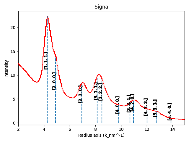
When you get the Azimuthal Integration now that things are calibrated it automatically accounts for the ewald sphere now and uses the non uniform axes.

calibrated_azim = au_dpeg.get_azimuthal_integral1d(npt=200, radial_range=(2, 15))
calibrated_azim.plot()
x = np.array(sim1d.reciprocal_spacing) * 10
y = [
    0.5,
] * len(x)
y0 = [
    0,
] * len(x)

hkl = [str(h) for h in sim1d.hkl]

offsets = np.vstack((x, y)).T
t = hs.plot.markers.Texts(
    offsets,
    texts=hkl,
    offset_transform="relative",
    horizontalalignment="left",
    verticalalignment="bottom",
    rotation=np.pi / 2,
    color="k",
)

calibrated_azim.add_marker(t)
lines = [[[l, 0], [l, 1]] for l in x]
v = hs.plot.markers.Lines(lines, transform="relative", linestyle="--")
calibrated_azim.add_marker(v)

  0%|          | 0/2 [00:00<?, ?it/s]
100%|██████████| 2/2 [00:00<00:00, 1357.38it/s]