Fast Plotting Tricks

Sometimes you want to quickly plot a diffraction pattern but things seem slow, this mostly happens with “large” data that is loaded Lazily.

There are a couple of different ways that plotting in hyperspy/pyxem can be slow:

1. The data is too large and the navigator is being recalculated every time you plot. (i.e. calling s.plot()

takes a long time to render)

2. Dragging the navigator is slow and laggy.

from pyxem.data import fe_multi_phase_grains
import numpy as np
import hyperspy.api as hs

s = fe_multi_phase_grains().as_lazy()

Pre Computing a Navaigator

To solve the first problem, you can:

1. Precompute the navigator using the hyperspy.api.signals.plot() method or the hyperspy._signals.LazySignal.compute_navigator() method which will compute the navigator and store it in the signal. This will make plotting faster.

s.compute_navigator()
print(s.navigator)

  0%|          | 0/2 [00:00<?, ?it/s]
100%|██████████| 2/2 [00:00<00:00, 1037.68it/s]
<Diffraction2D, title: , dimensions: (|20, 20)>

Setting a Navigator

2. You can also set the navigator directly using s.navigator = … if you have a navigator that you want to use. This is useful if a virtual image is created along with the signal when the data is acquired. This will also save the navigator in the metadata. This is similar to the :meth:`hyperspy._signals.LazySignal.compute_navigator`method of the signal and will be saved when the signal is saved.

dummy_navigator = hs.signals.Signal2D(np.ones((20, 20)))  # just a dummy navigator
s.navigator = dummy_navigator
# or
s.plot(navigator=dummy_navigator)

• 
• 

Using a Slider to Navigate

3. You also don’t need to plot the navigator every time you plot the signal. You can set navigator = “slider” to avoid plotting the navigator altogether and just use the sliders.

s.plot(navigator="slider")

VBox(children=(HBox(children=(Label(value='x', layout=Layout(width='15%')), IntSlider(value=0, description='index', max=19), BoundedFloatText(value=0.0, continuous_update=True, description='value', max=19.0, step=1.0), Label(value='px', layout=Layout(width='5%')))), HBox(children=(Label(value='y', layout=Layout(width='15%')), IntSlider(value=0, description='index', max=19), BoundedFloatText(value=0.0, continuous_update=True, description='value', max=19.0, step=1.0), Label(value='px', layout=Layout(width='5%')))), Checkbox(value=True, description='Continuous update')))

Using the QT Backend and Blitting

To solve the second problem, you can:

1. Use the Qt backend by running %matplotlib qt in a Jupyter notebook cell. This will make the navigator much more responsive using “blitting” which only updates the parts of the plot that have changed. Note that the QT backend is not available in Google Colab or when running in a Jupyter notebook on a remote server.

Using Shift + Click to Jump

2. You can use the Shift + Click feature to “Jump” to a specific location in the navigator. This is useful if you want to quickly move to a specific location in the navigator without dragging the navigator and loading all the data in between.

3. You can also set the navigator point using the axes_manager.indices attribute.

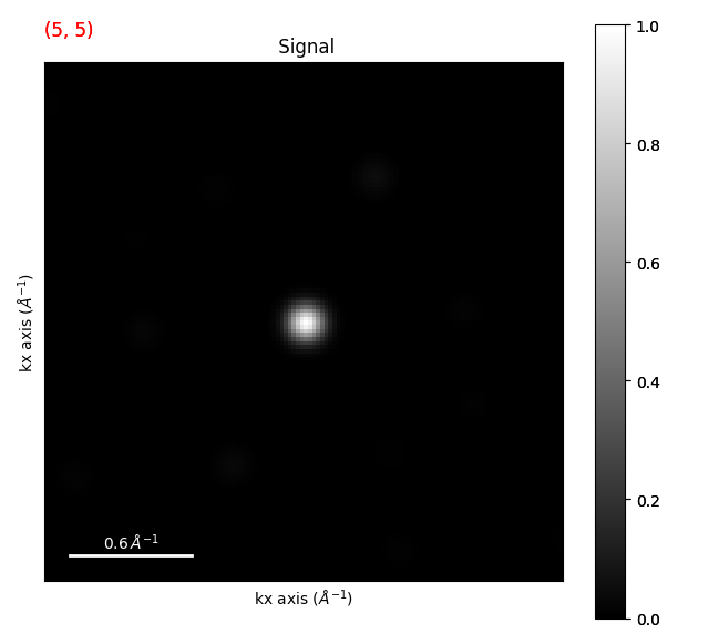
s.axes_manager.indices = (5, 5)  # jump to the center of the navigator
s.plot()

• 
• 

Saving the Data

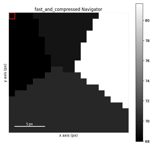
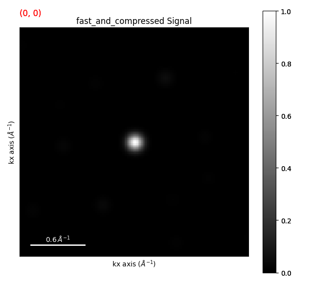
4. Finally, you can always consider saving the data in a more performant format like .zspy This will make loading the data faster which will in turn make plotting faster!

s.save("fast_and_compressed.zspy")

hs.load("fast_and_compressed.zspy").plot()  # reload the data and plot it

• 
• 

/home/docs/checkouts/readthedocs.org/user_builds/pyxem/envs/1139/lib/python3.11/site-packages/rsciio/zspy/_api.py:215: FutureWarning: The NestedDirectoryStore is deprecated and will be removed in a Zarr-Python version 3, see https://github.com/zarr-developers/zarr-python/issues/1274 for more information.
  store = zarr.storage.NestedDirectoryStore(

[                                        ] | 0% Completed | 194.67 us
[                                        ] | 0% Completed | 100.36 ms
[########################################] | 100% Completed | 200.78 ms