Electric Field Mapping

When we measure a change in the position of the electron beam on the camera, we are directly measuring that the electron beam has been deflected from the optic axis. In other words, the momentum of the electron beam in the xy plane has changed. Since electrons are charged particles, we can relate the electron’s momentum change to an electric field using the Lorentz force equation.

\[\frac{dp}{dt} = qE + \nu X B\]

This can be also expressed as:

\[\frac{m_0 \gamma | \nu |^2 \theta}{et} \approx E_{xy}\]

or solving for the electric field in the y (or x) direction:

\[\frac{m_0 \gamma | \nu |^2 \theta_y}{et} \approx E_{y}\]

Where \(m_0\) is the rest mass of the electron, \(\gamma\) is the Lorentz factor, \(| \nu |\) is the speed of the electron, \(e\) is the elementary charge, and \(t\) is the thickness of the sample and \(\theta_y\) is the deflection angle in the y direction.

Special thanks to Dr. Barnaby Levin for helping with the math and documentation for Electric Field Mapping.

from pyxem.data import simulated_pn_junction
import matplotlib.pyplot as plt
import hyperspy.api as hs

s = simulated_pn_junction()
s.calibration.convert_signal_units("mrad")
com = s.get_direct_beam_position(method="center_of_mass")
cal = com.pixels_to_calibrated_units()
ecal = cal.calibrate_electric_shifts(thickness=60)

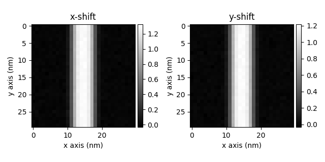
ecal.plot()

  0%|          | 0/31 [00:00<?, ?it/s]
 16%|█▌        | 5/31 [00:00<00:00, 45.37it/s]
 35%|███▌      | 11/31 [00:00<00:00, 50.55it/s]
 55%|█████▍    | 17/31 [00:00<00:00, 52.10it/s]
 74%|███████▍  | 23/31 [00:00<00:00, 52.89it/s]
 94%|█████████▎| 29/31 [00:00<00:00, 53.07it/s]
100%|██████████| 31/31 [00:00<00:00, 54.69it/s]

  0%|          | 0/33 [00:00<?, ?it/s]
100%|██████████| 33/33 [00:00<00:00, 9008.85it/s]

[<Axes: title={'center': 'x-shift'}, xlabel='x axis (nm)', ylabel='y axis (nm)'>, <Axes: title={'center': 'y-shift'}, xlabel='x axis (nm)', ylabel='y axis (nm)'>]

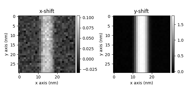
The shifts are new in units of mV/m, which is a common unit for electric fields. One thing that is important is to make sure that the camera x and y axes are aligned with the scan x and y axes. If they are not, you can use the rotate_beam_shifts method to align them.

rotated = ecal.rotate_beam_shifts(angle=45)  # Rotate the beam shifts by 45 degrees
rotated.plot()

[<Axes: title={'center': 'x-shift'}, xlabel='x axis (nm)', ylabel='y axis (nm)'>, <Axes: title={'center': 'y-shift'}, xlabel='x axis (nm)', ylabel='y axis (nm)'>]

Finding a Profile

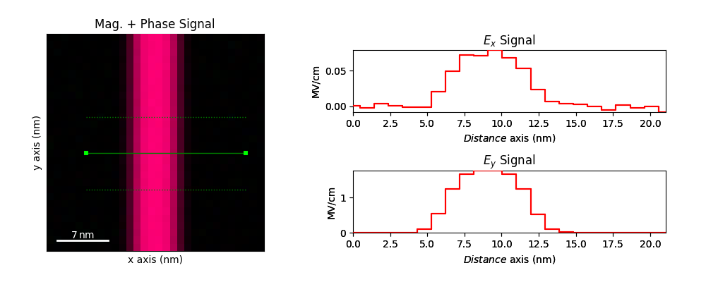
Now we can make a nice profile of the electric field using a line profile. Let’s make this interactive using a hyperspy ROI widgets. This should work best with the qt backend, although the ipympl backend should also work (hopefully). We could do this not interactively but this is a fun example of how to use hyperspy’s interactive tools.

# %matplotlib qt


fig = plt.figure(figsize=(10, 4))
gs = fig.add_gridspec(7, 7)
sub1 = fig.add_subfigure(gs[:, :3])
sub2 = fig.add_subfigure(gs[1:3, 3:])
sub3 = fig.add_subfigure(gs[4:6, 3:])
rot_signal = rotated.get_magnitude_phase_signal(add_color_wheel_marker=False)

rot_signal.metadata.General.title = "Mag. + Phase"
line = hs.roi.Line2DROI(x1=5, y1=16, x2=27, y2=16, linewidth=10)

E_x = line(rotated, axes=(0, 1)).isig[1].T
E_y = line(rotated, axes=(0, 1)).isig[0].T
E_x.set_signal_type("diffraction")
E_y.set_signal_type("diffraction")

E_x.metadata.General.title = "$E_x$"
E_y.metadata.General.title = "$E_y$"


E_x.axes_manager.signal_axes[0].name = "$Distance$"
E_y.axes_manager.signal_axes[0].name = "$Distance$"

rot_signal.plot(fig=sub1)
E_x.plot(fig=sub2)

E_y.plot(fig=sub3)


def get_profile(ind=0, out=None):
    res = line(rotated, axes=(0, 1)).isig[ind].T
    if out is not None:
        out.data[:] = res.data
        out.events.data_changed.trigger(obj=out)

    else:
        return res


# Connect the slices
for i, s in enumerate([E_x, E_y]):
    hs.interactive(
        get_profile,
        out=s,
        event=line.events.changed,
        recompute_out_event=line.events.changed,
        ind=i,
    )

line.add_widget(rot_signal)

<hyperspy.drawing._widgets.line2d.Line2DWidget object at 0x7588d81ea950>

sphinx_gallery_thumbnail_number = 5