Plotting a Diffraction Pattern

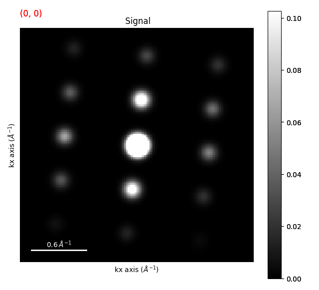
This is sometimes not as straightforward as it seems because you might have a zero beam that is too bright and regions of the diffraction pattern that are too dark.

from pyxem.data import fe_multi_phase_grains

mulit_phase = fe_multi_phase_grains()

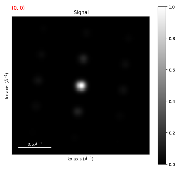
We can plot easily using the plot method. This will show the diffraction pattern but the plot is static and not interactive. Additionally, the zero beam is too bright and the high k values are too dark.

mulit_phase.plot()

• 
• 

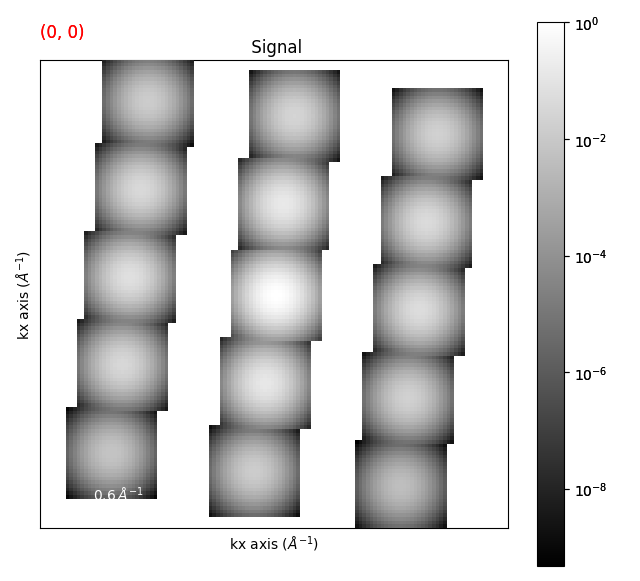
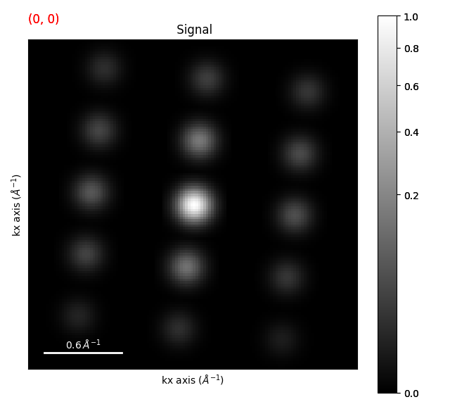
Plotting the diffraction pattern with a logarithmic scale can help to see the high k values But because most of the values are zero, the contrast is not great and is too stretched.

mulit_phase.plot(norm="log")

• 
• 

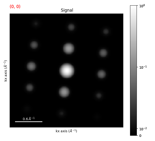
You can also use the symlog norm to plot the diffraction pattern with a logarithmic scale but with a linear scale around zero. This can be useful to see the zero beam and the high k values. additionally you can visualize negative and positive values as well.

mulit_phase.plot(norm="symlog")

• 
• 

We can also set vmin and vmax to control the contrast. This can be useful to see the high k values. A very useful feature is the ability to plot the diffraction pattern with vmax set to the 99th percentile. This sets the maximum value to the 99th percentile of the data. In general this works better than setting norm=’log’ if you have zero values in the diffraction pattern.

mulit_phase.plot(vmax="99th")

• 
• 

We can also use a gamma correction to control and optimize the contrast.

mulit_phase.plot(norm="power", gamma=0.4)

• 
• 

Note: that any of the plots are interactive if you add: %matplotlib ipympl or %matplotlib qt at the beginning of a Jupyter notebook cell. %matplotlib inline will make the plots static.